Work in progress. This post is being polished as we prepare the full release. The core ideas and figures are ready to read, and the code will be added soon.

Noise schedules are an essential design choice in diffusion models. They are also an awkward one. Everyone agrees that they matter, but the name hides several different decisions that are easy to mix together: how noise is added, which noise levels are sampled during training, how losses are weighted, and where the sampler later evaluates the trained model.

This is why schedule design often feels less like a principle and more like inherited infrastructure. Early DDPMs used a linear \(\beta_t\) schedule. Improved DDPM made cosine schedules a strong default. EDM separated many design choices and popularized a log-normal distribution over noise levels. More recent rectified-flow text-to-image models use logit-normal timestep sampling to bias training toward perceptually relevant scales. Each of these choices works somewhere. That is useful, but it also creates a practical problem: when starting a new diffusion project, we often inherit a schedule because it worked for a related setting, not because we know it is the right allocation for the current one.

If you are new to this topic, Sander Dieleman's post Noise schedules considered harmful is the best place to start. The useful lesson is not that schedules are unimportant. It is almost the opposite: schedules matter so much that using one word for several different objects can obscure what is actually being changed.

This post picks up from the adaptive end of that story. The question is not only which schedule family to choose before training. The harder question is why a fixed schedule should transfer at all. A schedule tuned for natural images may put training effort in a useful part of the path for CIFAR-10, FFHQ, or ImageNet. But if we move to binarized images, digitized pixels, DNA sequences, or language, there is no reason the same part of the path should remain the most useful.

Hidden variable

Training allocation

A schedule is not only a corruption curve. With the loss weight, it decides where optimization effort goes.

Reference signal

Entropy-rate profile

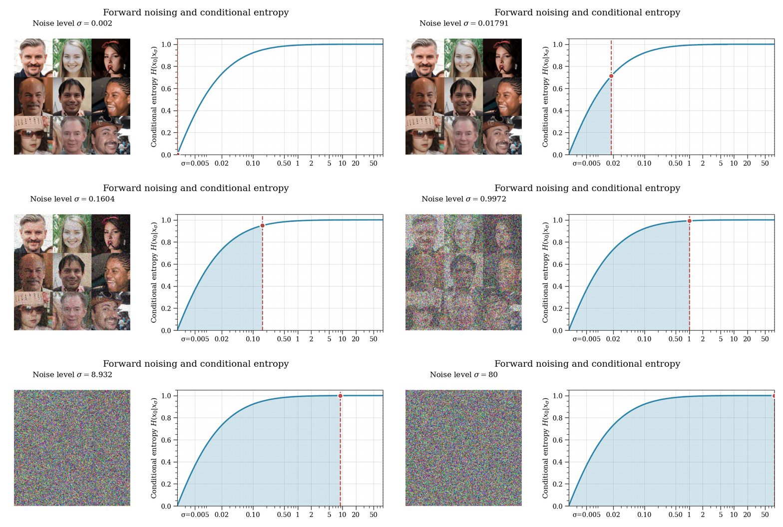
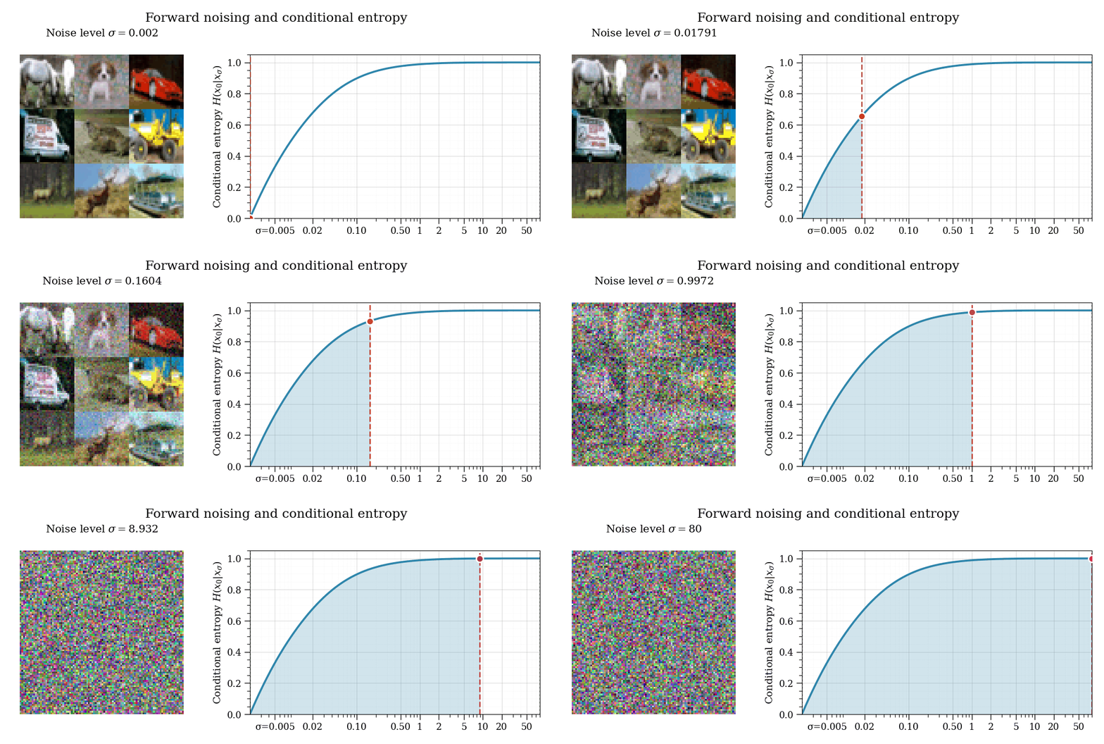
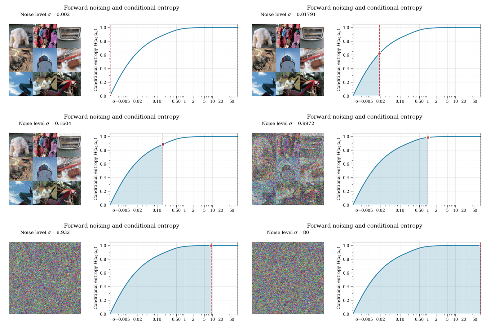
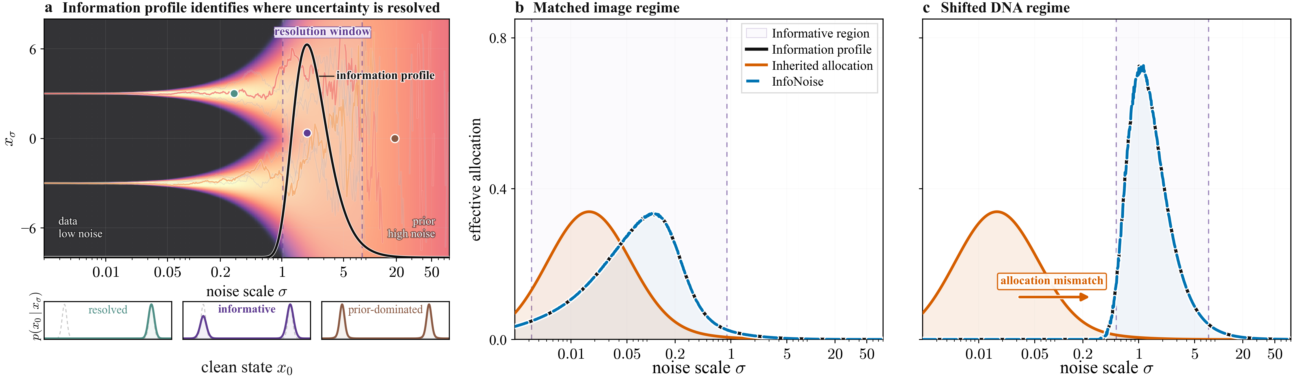
The useful region is where noisy observations reduce uncertainty about the clean sample fastest.

Minimal intervention

Adaptive sampler

InfoNoise changes the training-noise distribution while leaving the rest of the recipe fixed.

The community has repeatedly noticed a related pattern. Many successful schedules and weightings put extra pressure on intermediate noise levels: not the almost-clean endpoint, and not the pure-noise endpoint, but the region where signal and noise are both present. People describe this in different coordinates: middle timesteps, intermediate noise, logSNR near zero, perceptually relevant scales, or a transition region between signal-dominated and noise-dominated regimes.

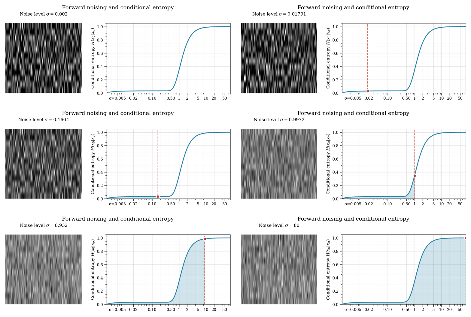
But “the middle” is not an invariant object. The middle of time is not necessarily the middle of \(\sigma\). The middle of \(\sigma\) is not necessarily the middle of log-SNR. And none of these coordinates tells us, by itself, where a particular dataset reveals information about its clean samples. A middle-biased schedule may be a good guess for one representation and a poor guess for another.

The object we want is therefore not the middle of a coordinate. It is the part of the corruption path where noisy observations actually reduce uncertainty about the clean sample. That is the point of InfoNoise: turn the vague intuition that “some intermediate region matters” into a data-dependent target for training allocation.

The schedule is not what the optimizer sees

A diffusion model is trained on many denoising problems. At one noise level, the model may only need to restore fine detail. At another, it may need to infer coarse structure. At very high noise, the observation may contain almost no usable information about the clean sample. The schedule decides how often these problems appear during training, but that is only part of the story.

The optimizer does not see a named schedule. It sees examples and weighted losses. If some noise levels are sampled often and their errors are weighted heavily, those regions dominate training. If other noise levels are sampled rarely or downweighted, they almost disappear. Once written this way, a schedule stops looking like a curve and starts looking like a distribution of training pressure.

Let \(u\) denote a coordinate along a corruption path, written in the data-to-noise direction. For an affine Gaussian path,

\[ x_u = a(u)x_0 + b(u)\epsilon, \qquad \epsilon \sim \mathcal N(0,I). \]

The coordinate \(u\) could be time, noise scale, log-SNR, or another monotone parameterization. At each \(u\), the model faces a different denoising problem. If the training sampler has density \(\pi(u)\), the loss has weight \(w(u)\), and the denoising risk at that noise level is \(R_x(u;\theta)\), then the training objective can be written as

\[ \mathcal L(\theta) = \int \underbrace{\pi(u)w(u)}_{\phi(u)} R_x(u;\theta)\,du . \]

The named schedule is not the only important object here. The product \[ \phi(u)=\pi(u)w(u) \] is the effective training allocation. It tells us how much the objective cares about each part of the denoising path after sampling and weighting have been taken into account.

This is the first useful reframing. If a schedule sweep improves a model, it may not be because one corruption curve is magically better than another. It may be because the sweep moved training effort toward a more useful part of the path.

Allocation view. Noise schedules are usually drawn as curves, but during training they behave more like a budget. They help decide which denoising problems receive updates. The question is where that budget should go.

Allocation needs a target

Once we look at schedules this way, the next question is unavoidable. If training effort can be moved around the path, what should it be moved toward?

Raw denoising loss is not enough. A noise level can have high loss because it is important, but it can also have high loss because the problem is nearly impossible. A low-loss region may be easy because the model has already learned it, or because there was little uncertainty there to resolve in the first place.

We instead look at conditional entropy:

\[ H(X_0 \mid X_u). \]

This quantity asks how much uncertainty remains about the clean sample \(X_0\) after observing the noisy sample \(X_u\). At high noise, the observation says little about \(X_0\). At low noise, it almost reveals \(X_0\). The interesting region is where this uncertainty changes fastest.

\[ \rho^\star(u) \propto \left| \frac{d}{du}H(X_0 \mid X_u) \right|. \]

We call this the information profile. It is not “the middle” of an arbitrary coordinate. It is the part of the path where noisy observations reduce uncertainty about the clean sample most rapidly.

For affine Gaussian corruption paths, this profile is connected to Bayes-optimal denoising error through the I-MMSE identity. If the signal-to-noise ratio is \[ \gamma(u)=\frac{a(u)^2}{b(u)^2}, \] then, up to normalization,

\[ \rho^\star(u) = \frac{1}{2}|\gamma'(u)|\,\mathrm{MMSE}(u). \]

In VE coordinates, where \[ x_\sigma=x_0+\sigma\epsilon, \] the same relationship becomes

\[ \frac{d}{d\sigma}H(X_0\mid X_\sigma) = \frac{\mathrm{MMSE}(\sigma)}{\sigma^3}. \]

The MMSE tells us how much uncertainty remains. The entropy rate tells us where uncertainty is being resolved. That distinction is the reason this profile is useful as an allocation target: it does not simply chase large errors; it identifies where the denoising problem is changing.

The decision window

Allocation only helps if it lands in the informative region. (a) In a two-state Gaussian channel, the posterior changes most quickly in a narrow decision window. (b) In mature image settings, inherited schedules often already place effort near this region. (c) Under representation or modality shift, the information profile can move while the inherited allocation stays put.

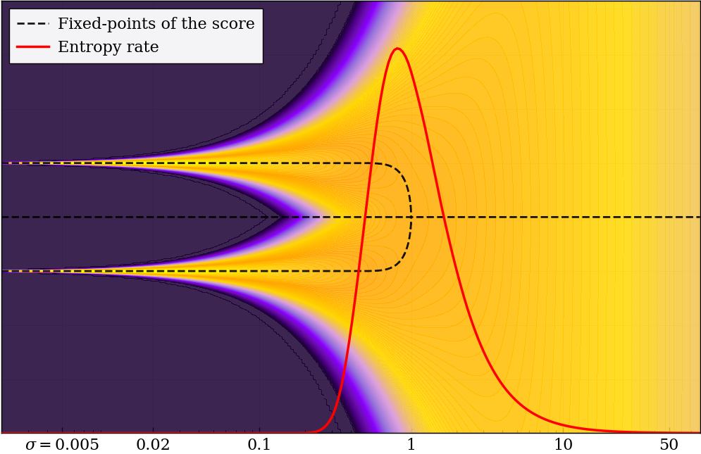
The toy example shows the local mechanism. At high noise, the posterior averages over possible clean states. At low noise, the clean state has essentially been decided. Between these regimes, the observation begins to select one explanation over another. The entropy-rate peak marks this decision window.

This is close to what people often mean informally when they say that intermediate noise levels matter. But the figure also shows why the informal version is not enough. The useful region is not defined by being halfway along a chosen axis. It is defined by the posterior changing quickly.

The optimal denoiser changes most in the transition region. In the toy problem, the optimal denoiser moves from averaging over possible clean samples to committing to one branch. The CIFAR-10 diagnostic shows the same qualitative behavior in a real image setting: the optimal denoised prediction changes most in an intermediate region, not uniformly across the path.

This also connects to our earlier work on spontaneous symmetry breaking in diffusion models. In generation, structure is not recovered uniformly along the reverse trajectory. There are regimes where samples remain ambiguous, and regimes where they commit. Here we ask the training-side version of the same question: if the denoising problem changes unevenly along the path, why should training effort be inherited from a fixed schedule?

A schedule sweep is allocation search

The DNA experiment makes the allocation view concrete. We keep the objective, weighting, prediction parameterization, model, optimizer, sampler, and evaluation protocol fixed. The only change is \(P_{\mathrm{mean}}\), the location parameter of the EDM log-normal training distribution. Moving this parameter shifts training effort along \(\log\sigma\).

A schedule sweep repeatedly searches for the right allocation. Sweeping the EDM \(P_{\mathrm{mean}}\) parameter moves training effort along the DNA corruption path. Allocations closer to the information profile reach the target Sei-FID with fewer processed examples. InfoNoise moves toward this region online, without training a sweep of fixed schedules.

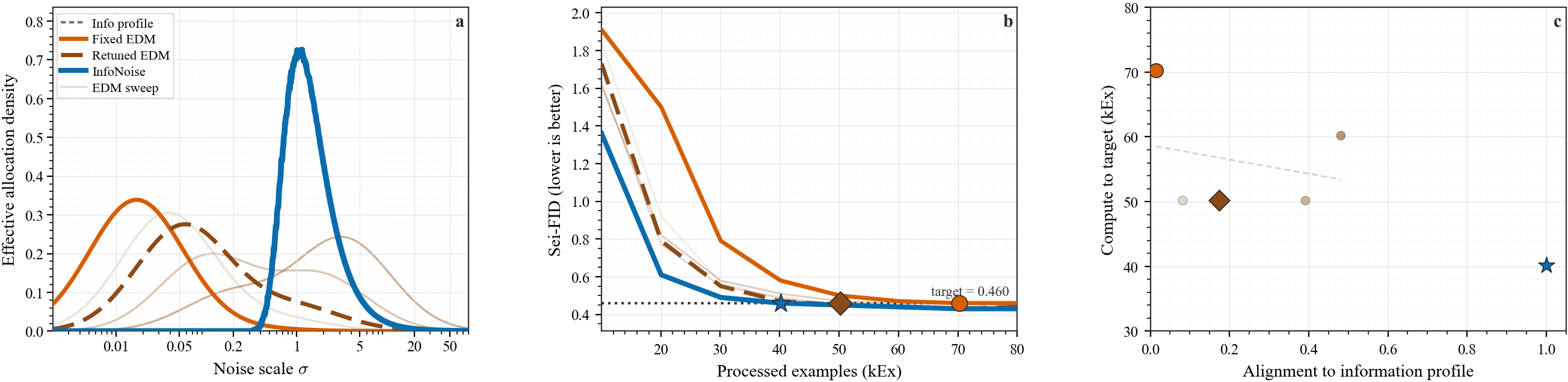
This is the practical motivation. If the useful region were known in advance, we could tune a fixed schedule to place mass there. But in a new representation or modality, that region is often exactly what we do not know. A fixed schedule guesses once. A sweep guesses repeatedly. InfoNoise uses a signal measured during training to update the guess.

InfoNoise only moves the sampler

InfoNoise is deliberately narrow. It does not change the architecture, objective, loss weighting, prediction parameterization, optimizer, EMA, augmentations, inference sampler, or evaluation budget. It changes only the distribution from which training noise levels are sampled.

During training, the model already computes denoising losses. InfoNoise tracks these losses across noise levels, converts them into an online estimate of the information profile, and uses that estimate to update the training noise density:

\[ \pi(u) \quad\longrightarrow\quad \pi_{\mathrm{InfoNoise}}(u). \]

The adapted density defines a CDF, and inverse-CDF sampling draws new noise levels from it. With \(w(u)\) unchanged, moving \(\pi(u)\) moves the effective allocation

\[ \phi(u)=\pi(u)w(u). \]

• Track denoising losses across corruption levels.
• Estimate an online information profile \(\widehat{\rho}(u)\).
• Adapt the training-noise density \(\pi_{\mathrm{InfoNoise}}(u)\).
• Sample new training noise levels by inverse CDF while keeping the rest of training fixed.

Adaptive sampling without changing the denoising objective. InfoNoise estimates an information profile online, converts it into a training-noise density, and samples new noise levels through the inverse CDF. The intervention is an allocation change, not a new prediction target.

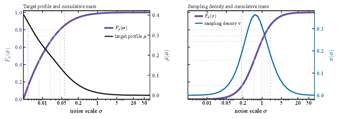
This is the first step toward adaptive schedule design in the training sense. The schedule is no longer chosen once, before the distribution of denoising difficulty is known. It is adjusted using a data-dependent signal from the current training run.

What changes in practice

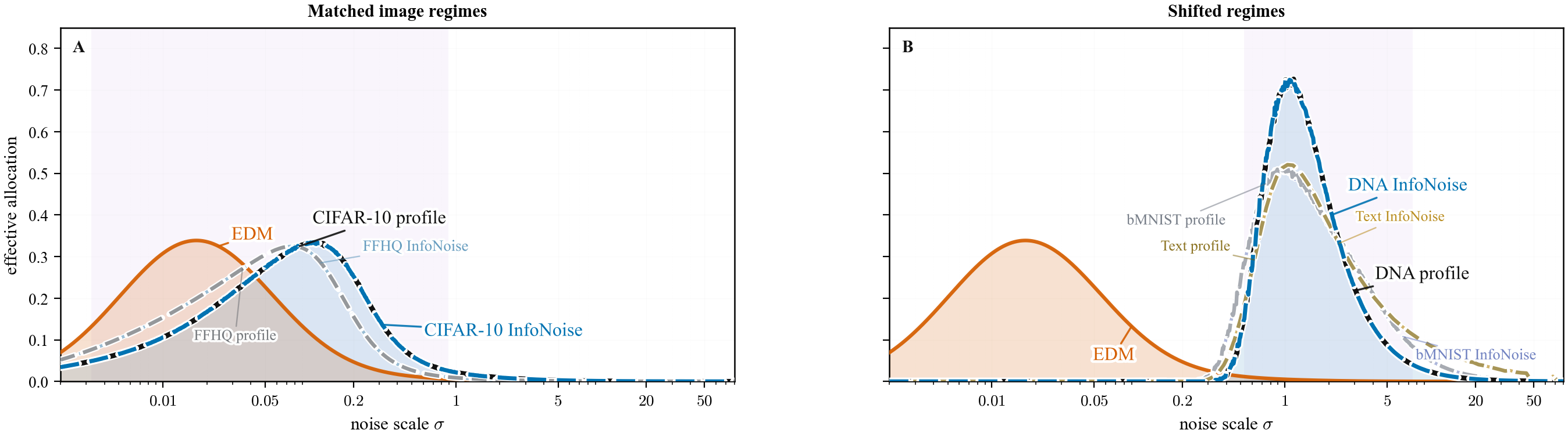
The empirical pattern is intentionally asymmetric. In standard image regimes, fixed schedules have already been tuned extensively. There, InfoNoise mostly recovers a similar allocation and matches strong baselines. That is not a failure of adaptivity; it is what should happen when the inherited allocation is already good.

The larger gains appear when the inherited allocation is mismatched. In binarized images, digitized images, DNA, and language, the informative region shifts. A schedule tuned for one regime can spend too many updates elsewhere. InfoNoise helps because it follows the measured information profile rather than assuming the image-tuned allocation still applies.

Dataset	Metric	NFE	LogU	Cos	FM	EDM	KG	InfoNoise
Fashion	FID down	35	2.75	1.76	1.93	1.78	1.82	1.71
CIFAR uncond.	FID down	35	5.93	2.16	2.31	2.04	2.00	1.98
CIFAR cond.	FID down	35	4.45	2.11	2.13	1.85	1.84	1.84
FFHQ 64	FID down	79	4.68	2.69	2.72	2.53	2.54	2.53
bMNIST	FID down	35	0.63	0.52	0.38	0.53	0.38	0.33
bFashion	FID down	35	1.10	1.20	0.80	0.94	1.22	0.69
Digit. CIFAR	FID down	255	17.30	-	-	9.90	-	3.10
DNA	Sei-FID down	35	0.61	0.42	0.44	0.45	0.43	0.42
OWT-2	MAUVE up	127	0.68	-	-	0.83	-	0.87

This table should not be read as saying that adaptive schedules always beat hand-designed schedules. The cleaner reading is: when a mature fixed schedule is already aligned, InfoNoise preserves that allocation; when the information profile moves, InfoNoise follows it.

Schedule transfer works when the profile stays put. In matched image regimes, inherited schedules already allocate effort near the measured information profile. Under representation or modality shift, the profile moves away from the inherited allocation. This is where adaptive training noise sampling matters most.

What this does not solve

InfoNoise is not a complete theory of diffusion schedules. It adapts the training noise distribution, not the whole training system. The loss weight, prediction parameterization, architecture, optimizer, sampler, guidance mechanism, and endpoint choices still matter. Training allocation and inference discretization are related, but they are not the same problem.

The online estimate also has practical degrees of freedom: warm-up, smoothing, binning, calibration, and boundary behavior near deterministic limits. These are not cosmetic details. They affect how quickly the sampler should move and how much noise should be trusted in the profile estimate.

The point is therefore not that schedule design disappears. The point is that one expensive part of schedule design can be made explicit and data-adaptive. Instead of repeatedly sweeping a schedule family to find where effort should go, we can estimate where uncertainty is being resolved and allocate training there.

How to think about schedules after this

The allocation view changes the checklist. When a schedule works or fails, ask:

• Which object changed: the corruption path, the training sampler, the loss weight, the prediction target, or the inference grid?
• After weighting, where is the effective allocation \(\phi(u)=\pi(u)w(u)\)?
• Does that allocation overlap the conditional-entropy-rate profile of the current data?
• If a schedule parameter is swept, is the sweep mainly moving mass along log-SNR?
• If the representation or modality changed, should the informative region be expected to stay in the same place?

A fixed schedule is not wrong by default. It is wrong when it allocates training effort to the wrong part of the denoising path. For familiar image settings, years of empirical tuning have often already found a good allocation. For new domains, that inherited allocation is a guess.

InfoNoise replaces that guess with a measured target: the rate at which noisy observations reduce uncertainty about the clean sample. That is the practical shift. Noise-schedule design becomes less about choosing a named curve, and more about asking where the current data actually become informative.

Further reading

• InfoNoise paper
• Sander Dieleman: Noise schedules considered harmful
• DDPM: Denoising Diffusion Probabilistic Models
• Improved DDPM
• EDM: Elucidating the Design Space of Diffusion-Based Generative Models
• Efficient Diffusion Training via Min-SNR Weighting Strategy
• Common Diffusion Noise Schedules and Sample Steps are Flawed
• Scaling Rectified Flow Transformers for High-Resolution Image Synthesis
• The I-MMSE identity